From Monte Carlo to Stockholm

Simulating Your Way to Smart Apartment Investments

Monte Carlo, Monaco. Photo by Rishi

I have to admit, I often struggle with decision anxiety. I can hardly decide what to eat for lunch, so how am I supposed to make major financial decisions, like investing in a new apartment?

Recently, “we” (my girlfriend) decided we should move to a larger apartment since “we” (i helped) just had a baby. This meant we had to invest and transfer a significant amount of money between real estate properties.

This got me thinking. We did some budgeting and consulted our bank connections, but that was about it. People make big investment decisions many times throughout their lives, often without a complete picture of the possible outcomes.

The Monte Carlo Simulation

Stockholm, Sweden. Photo by Ana Bórquez

Today kids, we are going to use a Monte Carlo Simulation to estimate potential outcomes when buying an apartment in Stockholm, Sweden. A Monte Carlo Simulation involves running multiple simulations with random values to capture a wide range of possible outcomes.

Here is an example rolling a six-sided die:

• Define the Problem:

  • You want to estimate the mean value when rolling a six-sided die.

• Set Up the Simulation:

  • You will generate random numbers between 1 and 6 to simulate rolling the die multiple times.

• Run the Simulation:

  • Simulate rolling the die 10 times.

• Analyze the Results:

  • Calculate the mean of these 10 simulated rolls.

This is a chart that shows the two first simulation result out of 10 and also the mean value out of all simulations.

Our Experiment

In our experiment we are going to look at how the investment looks over a 10 year period, so each simulation is has 10 “steps”, one for each year.

First, we need some numbers. The price of a 3-bedroom apartment in downtown Stockholm is around $800,000 (DAMN!). Since we don't have $800,000 in cash, we could either rob a bank (high risk) or take out a mortgage. Let's go with the mortgage.

The Data

We also need current and historical interest rates and mean annual returns for apartment investments in Sweden. These can be found on any Swedish bank's website and the Swedish Real Estate Agent Statistics website, respectively. Both datasets span from 1997 to 2023, ensuring that our calculations for mean and standard deviation are consistent over the same time period.

I just uploaded both data sets to ChatGPT and told “it” to give me the mean and std for both data sets.

We need historical data to include the standard deviation (std) in our simulation, introducing randomness for each run. For example, one run might have an interest rate of 6% instead of 4%, with the standard deviation setting upper and lower limits on these fluctuations.

The Apartment

• Price: $800,000

• Mean annual return: 7.96%

• Standard deviation of annual return: 8.88%

The Mortgage

• Principal (total credit): $750,000

• Mean interest rate: 4.21%

• Standard deviation of interest rate: 1.67%

We will simulate this investment over the first 10 years, running the simulation 100,000 times and plotting some interesting data.

Apartment Value Simulation

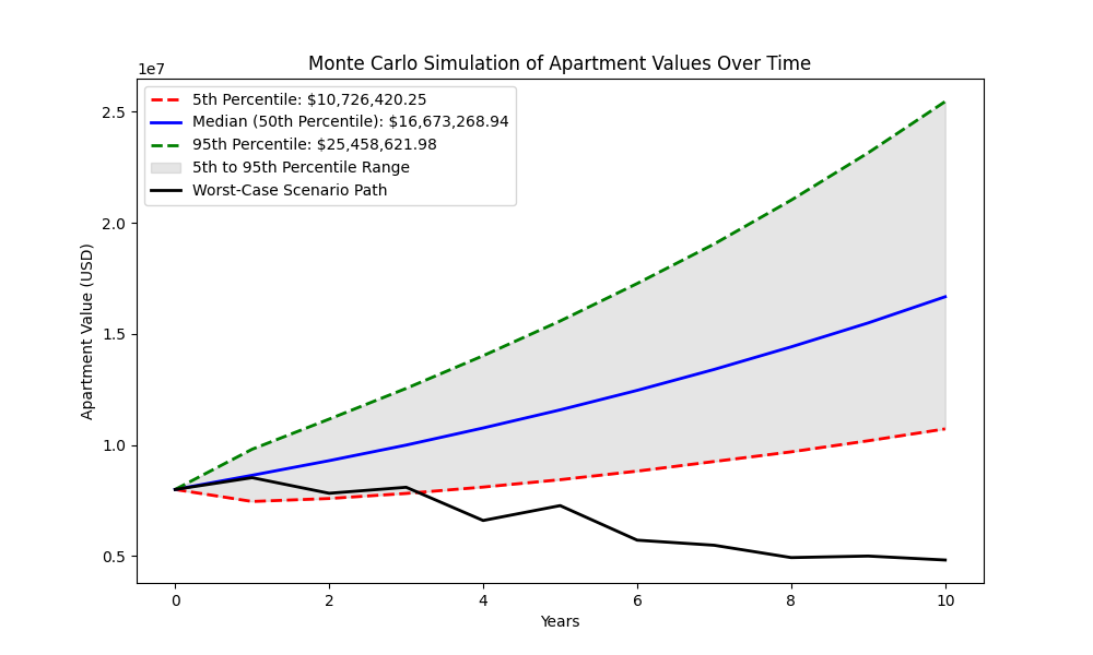
Chart of the potential apartment values over a 10 year period

• 5th Percentile: $10,726,420

• Median (50th Percentile): $16,673,268

• 95th Percentile: $25,458,621

The 95th percentile represents optimistic outcomes, the 5th percentile represents pessimistic outcomes, and the blue line represents the mean outcome. The black line is the absolut worst scenario. The gray area represents all other possible outcomes from the simulation.

From this, I can see that if things go wrong, it could be living on the streets within 5 years, but the likelihood of that is less then 1%. Most outcomes are positive, and even the 5th percentile eventually indicates a good investment over a 10-year horizon.

Realistically, the median value is the most likely outcome, indicating that this is a very good investment ($800,000 USD → $1,600,000 USD)

Interest Rate Simulation

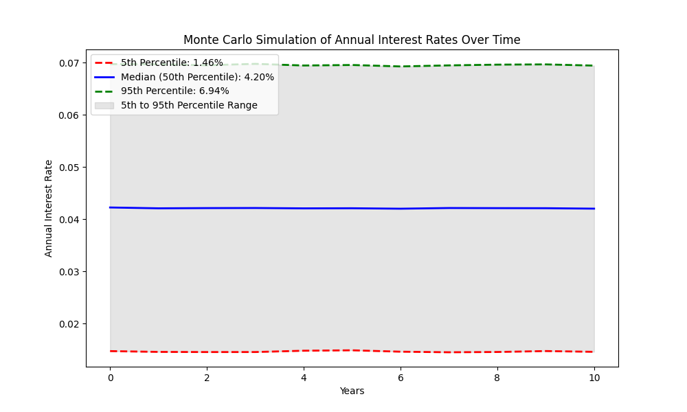
Chart of the potential interest rate over a 10 year period

This chart shows potential interest rates. Here, I prefer lower interest rates, so I am rooting for the 5th percentile. But most likely the interest rate will be around 4.20% (hehe).

Total Investment Value Simulation

Chart of the potential apartment values minus the cost of the loan

This chart shows the actual value of the apartment minus the total cost of the loan (interest rates). It suggests that I will likely make a good investment if I plan to own the apartment for at least 10 years. The mean here is $16,389.001, that is a 100% return on my initial investment.

Histogram of the potential apartment values minus the cost of the loan

Looking at the simulation using a histogram helps us see where most final values end up for all our simulations. The height of each bar represents how many simulations ended up in that bin. It also helps us spot how the outliers are distributed (5th and 95th percentiles). The 95th percentile has a longer tail, indicating more variation in the optimistic outcomes.

Conclusion

While this simulation might not capture the entire truth, it provides a good overview of potential outcomes and what to expect. Buying an apartment in Stockholm, Sweden, seems like a pretty stable investment.

We could create a much more complex simulation that also considers our income, amortization, inflation, and incorporate more accurate data, such as the specific property values for the district we plan to move to.

The code

from dataclasses import dataclass
import matplotlib.pyplot as plt
import numpy as np


@dataclass
class Investment:
    price: float
    annual_return_mean: float
    annual_volatility: float


@dataclass
class Simulation:
    years: int
    n: int


@dataclass
class Loan:
    principal: float
    interest_rate_mean: float
    interest_rate_volatility: float


def run_simulation_with_worst_case_tracking(
    sim: Simulation, investment: Investment, loan: Loan
):
    final_values = np.zeros((sim.n, sim.years + 1))
    interest_rates = np.zeros((sim.n, sim.years + 1))
    apartment_values = np.zeros((sim.n, sim.years + 1))

    worst_case_path = None
    min_final_value = float("inf")

    for step in range(sim.n):
        investment_value = investment.price
        apartment_value = investment.price
        final_values[step, 0] = investment_value
        apartment_values[step, 0] = apartment_value

        # Set initial interest rate
        initial_interest_rate = np.random.normal(
            loan.interest_rate_mean, loan.interest_rate_volatility
        )
        interest_rates[step, 0] = initial_interest_rate

        for year in range(1, sim.years + 1):
            annual_return = np.random.normal(
                investment.annual_return_mean, investment.annual_volatility
            )
            apartment_value *= 1 + annual_return

            # Calculate the annual loan interest payment
            annual_interest_rate = np.random.normal(
                loan.interest_rate_mean, loan.interest_rate_volatility
            )
            annual_interest_payment = loan.principal * annual_interest_rate

            # Record the interest rate
            interest_rates[step, year] = annual_interest_rate

            # Subtract the loan interest payment from the investment value
            investment_value = apartment_value - annual_interest_payment

            # Ensure investment value does not drop below zero
            # investment_value = max(investment_value, 0)

            final_values[step, year] = investment_value
            apartment_values[step, year] = apartment_value

        # Track the worst-case scenario
        if final_values[step, -1] < min_final_value:
            min_final_value = final_values[step, -1]
            worst_case_path = apartment_values[step, :]

    return final_values, interest_rates, apartment_values, worst_case_path


def plot_worst_case_scenario(worst_case_path, filename="worst_case_plot.png"):
    plt.figure(figsize=(10, 6))
    years = np.arange(len(worst_case_path))

    plt.plot(
        years,
        worst_case_path,
        color="black",
        linestyle="solid",
        linewidth=2,
        label="Worst-Case Scenario Path",
    )

    plt.title("Worst-Case Scenario for Apartment Values Over Time")
    plt.xlabel("Years")
    plt.ylabel("Apartment Value (USD)")
    plt.legend(loc="upper left")
    plt.savefig(filename)
    plt.close()


# Example usage with Swedish housing market and loan
investment = Investment(
    price=8000000, annual_return_mean=0.0796, annual_volatility=0.0888
)
simulation = Simulation(years=10, n=100000)
loan = Loan(
    principal=7500000, interest_rate_mean=0.0421, interest_rate_volatility= 
)  # Example loan parameters

# Run simulation with worst-case tracking
values, interest_rates, apartment_values, worst_case_path = (
    run_simulation_with_worst_case_tracking(simulation, investment, loan)
)

# Plot worst-case scenario
plot_worst_case_scenario(worst_case_path)

# Display the plot
plt.figure(figsize=(10, 6))
years = np.arange(len(worst_case_path))

plt.plot(
    years,
    worst_case_path,
    color="black",
    linestyle="solid",
    linewidth=2,
    label="Worst-Case Scenario Path",
)

plt.title("Worst-Case Scenario for Apartment Values Over Time")
plt.xlabel("Years")
plt.ylabel("Apartment Value (USD)")
plt.legend(loc="upper left")
plt.show()


def plot_apartment_values_with_worst_case(
    apartment_values,
    worst_case_path,
    filename="apartment_value_with_worst_case_plot.png",
):
    plt.figure(figsize=(10, 6))

    # Calculate percentiles
    p5 = np.percentile(apartment_values, 5, axis=0)
    p50 = np.percentile(apartment_values, 50, axis=0)
    p95 = np.percentile(apartment_values, 95, axis=0)

    years = np.arange(apartment_values.shape[1])

    plt.plot(
        years,
        p5,
        color="red",
        linestyle="dashed",
        linewidth=2,
        label=f"5th Percentile: ${p5[-1]:,.2f}",
    )
    plt.plot(
        years,
        p50,
        color="blue",
        linestyle="solid",
        linewidth=2,
        label=f"Median (50th Percentile): ${p50[-1]:,.2f}",
    )
    plt.plot(
        years,
        p95,
        color="green",
        linestyle="dashed",
        linewidth=2,
        label=f"95th Percentile: ${p95[-1]:,.2f}",
    )

    plt.fill_between(
        years, p5, p95, color="gray", alpha=0.2, label="5th to 95th Percentile Range"
    )

    # Plot worst-case scenario
    plt.plot(
        years,
        worst_case_path,
        color="black",
        linestyle="solid",
        linewidth=2,
        label="Worst-Case Scenario Path",
    )

    plt.title("Monte Carlo Simulation of Apartment Values Over Time")
    plt.xlabel("Years")
    plt.ylabel("Apartment Value (USD)")
    plt.legend(loc="upper left")
    plt.savefig(filename)
    plt.close()


# Plot apartment values with worst-case scenario
plot_apartment_values_with_worst_case(apartment_values, worst_case_path)

# Display the plot
plt.figure(figsize=(10, 6))
years = np.arange(apartment_values.shape[1])

p5 = np.percentile(apartment_values, 5, axis=0)
p50 = np.percentile(apartment_values, 50, axis=0)
p95 = np.percentile(apartment_values, 95, axis=0)

plt.plot(
    years,
    p5,
    color="red",
    linestyle="dashed",
    linewidth=2,
    label=f"5th Percentile: ${p5[-1]:,.2f}",
)
plt.plot(
    years,
    p50,
    color="blue",
    linestyle="solid",
    linewidth=2,
    label=f"Median (50th Percentile): ${p50[-1]:,.2f}",
)
plt.plot(
    years,
    p95,
    color="green",
    linestyle="dashed",
    linewidth=2,
    label=f"95th Percentile: ${p95[-1]:,.2f}",
)

plt.fill_between(
    years, p5, p95, color="gray", alpha=0.2, label="5th to 95th Percentile Range"
)

# Plot worst-case scenario
plt.plot(
    years,
    worst_case_path,
    color="black",
    linestyle="solid",
    linewidth=2,
    label="Worst-Case Scenario Path",
)

plt.title("Monte Carlo Simulation of Apartment Values Over Time")
plt.xlabel("Years")
plt.ylabel("Apartment Value (USD)")
plt.legend(loc="upper left")
plt.show()